Profiling coupled simulations

The first challenge one faces when creating a coupled simulation is getting it to run correctly. Once the model is running and producing results however, the question often becomes how to make it run faster, so as to be able to do science more efficiently. The model needs to be optimised.

The first step of optimisation is measurement: how much compute time does the model spend on what? Without measurement, you end up optimising parts that don’t contribute significantly to the total run time, thus making little progress.

Measuring and optimising individual submodels is outside of the scope of MUSCLE3. This should be done at the level of the individual model, using profilers like gprof or perf or TotalView, and there isn’t much MUSCLE3 can contribute. In a coupled simulation however, you first need to know which of the coupled models takes the most compute time and should therefore be optimised, and this MUSCLE3 can help with.

A MUSCLE3 simulation consists of a set of submodels, which during the simulation spend some of their time computing, some of it waiting for inputs to arrive from other submodels, and some of it transferring data. The communication activities are done through libmuscle, and computing (and internal communication, if the model is parallelised) takes place in between them. During each run, libmuscle will measure when each external communication takes place, how much time was spent waiting, and how much time was spent transferring the data. This information is collected centrally and saved to a file, which you can then analyse to discover where the coupled simulation can best be optimised.

Configuring profiling

Profiling is enabled by default, so you do not have to do anything to get MUSCLE3 to produce profiling data. For typical coupled simulations consisting of only a few instances that do not communicate very often, this should not affect the simulation performance. If you have a simulation with very many instances which communicate intensively, then the overhead of sending all that information to the central database can become significant.

If that is the case, then you should do your profiling with a smaller number of instances, and disable profiling for the large run to avoid the overhead. Profiling can be disabled by setting the setting muscle_profile_level to none in the yMMSL file. To enable profiling, set it to all, or don’t set it at all. Just like for other settings, this can be set per-instance as well, to selectively collect profiling information from part of the simulation.

The profiling database

After a MUSCLE3 simulation is done, you will find a file called performance.sqlite in the run directory, next to the main log file. This file is a database containing several tables with performance information about the run.

This information can be analysed in three ways: 1) through the muscle3 profile command, 2) via the libmuscle.ProfileDatabase class in Python, and 3) directly via sqlite3 from the shell or from Python. All three are described here.

Plotting statistics from the command line

The simplest way of examining performance data gathered by MUSCLE3 is through the muscle3 profile command from the shell. If you have done a run, then you should have a run directory containing a performance.sqlite file. If you have MUSCLE3 available in your environment (only the Python installation is needed) then you have the muscle3 profile command available to show per-instance and per-core statistics as well as a timeline of events.

Per-instance time spent

muscle3 profile --instances /path/to/performance.sqlite

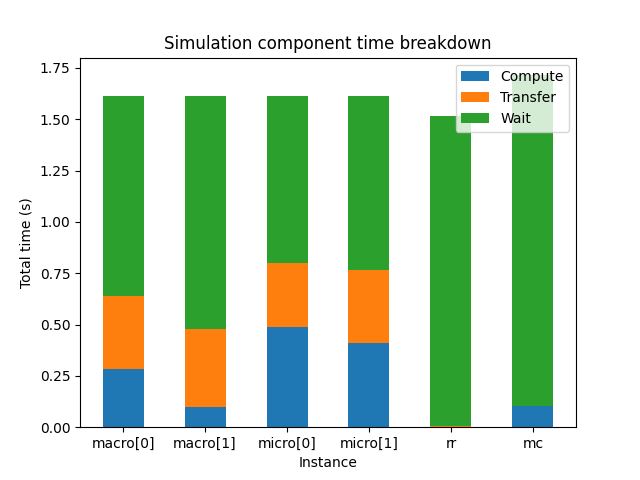
With --instances or -i, the plot will show for each instance how much time it spent in total on computing, communicating and waiting. This plot gives an idea of where most of the computing is done, and which components you need to optimise to get an answer sooner.

In many models, you will find that there’s one component that takes up most of the compute time, and others that spend most of their time waiting and then do a little bit of computing. This is not necessarily wasteful, it may simply be that most of the work is in that one component. Of course it does mean that if you want to get your result faster, you should focus your efforts on the component that takes the most time.

This works fine for relatively simple models, but there are some caveats to take into account. First, model components may use different amounts of resources. A component that runs 10% of the time, but uses 100 cores, uses a lot more energy than one that runs 90% of the time on a single core. On the other hand, if you are interested in getting an answer more quickly, then you should optimise the single-core model first.

If you are running on HPC, then you most likely have a fixed budget of core hours or system billing units (SBUs), and reducing SBU usage may be of interest. In the above scenario, both models are actually candidates for optimisation in this case. If you can speed up the parallel model so that it can run as fast on fewer cores then that potentially saves many SBUs. But speeding up the single-thread model also helps, because even if the cores that the parallel model runs on aren’t used, they’re still allocated and you’re still paying for them.

If all your models spend most of their time communicating, then your models do relatively little work in between sending and receiving messages. In that case, either MUSCLE3 needs to be optimised, or perhaps your coupling is simply too tight to do over a network connection and you should consider integrating the codes directly.

Resource usage

muscle3 profile --resources /path/to/performance.sqlite

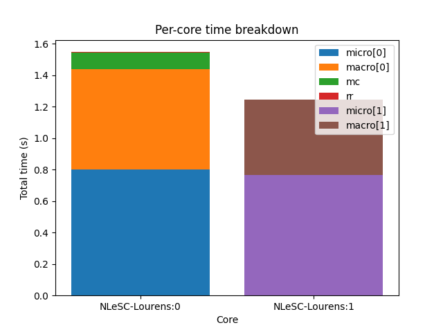
If you are running on a large computer, then it may be interesting to see how you are using the resources allocated to you. The command muscle3 profile --resources performance.sqlite will produce a plot showing for each core how much time it spent running the various instances (-r for short also works). This gives an idea of which component used the most resources, and tells you what you should optimise if you’re trying to reduce the number of core hours spent.

The total time shown per core doesn’t necessarily match the total run time, as cores may be idle during the simulation. This can happen for example if components A and B alternate execution but use different numbers of cores. MUSCLE3 will automatically detect that A and B alternate and assign overlapping sets of cores so as to use them optimally, but if A uses 10 and B uses 15 cores, then inevitably 5 cores will be idle while A is running.

Event timeline

muscle3 profile --timeline /path/to/performance.sqlite

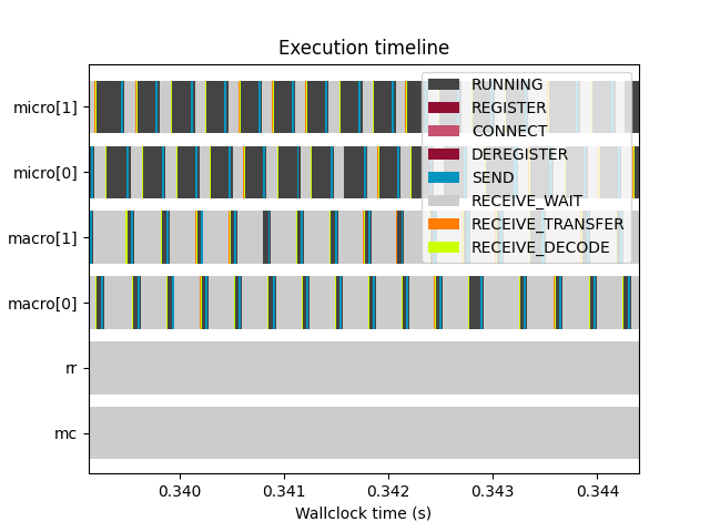
If you really want to get into the details, --timeline or -t shows a timeline of profiling events. This visualises the raw data from the database, showing exactly when each instance sent and received data, when it was waiting for input, and when it computed. The meaning of the event types shown is as follows:

REGISTER

The instance contacted the manager to share its location on the network, so that other instances can communicate with it.

CONNECT

The instance asked the manager who to communicate with, and set up connections to these other instances.

RUNNING

The instance was running, meaning that it was actively computing or doing non-MUSCLE3 communication.

SHUTDOWN_WAIT

The instance was waiting to receive the information it needed to determine that it should shut down, rather than run the reuse loop again.

DISCONNECT_WAIT

The instance was waiting for the instances it communicates with to acknowledge that it would be shutting down. This may take a while if those other instances are busy doing calculations or talking to someone else.

SHUTDOWN

The instance was shutting down its MUSCLE3 communications.

DEREGISTER

The instance contacted the manager to say that it was ending it run.

SEND

The instance was sending a message. This includes encoding the sent data and putting it in a queue, ready to be picked up by the receiver. The actual transfer is done in the background, and is excluded here.

RECEIVE_WAIT

The instance was waiting for another instance to send it a message.

RECEIVE_TRANSFER

The instance was receiving data from another instance. Note that because of the way operating systems work, transfer of the very first bit of data (the first network packet) is counted with RECEIVE_WAIT, so that for very small messages this may seem to take no time at all.

RECEIVE_DECODE

The received data were being decoded and turned into Python objects or Data objects.

On most installations, this plot is interactive, so be sure to use the pan and zoom buttons at the bottom of the window to explore the data.

The plots here are implemented using matplotlib, which doesn’t do very well displaying large numbers of events. To avoid endless rendering, the data will be truncated if it is too large, so that you can at least see the start of the simulation. If you find yourself running into this limitation, please make an issue on GitHub and we’ll increase the priority on improving this.

Analysis with Python

If you want to get quantitative data, or just want to make your own plots, then you can use MUSCLE3’s Python API. It contains several useful functions for extracting information and statistics from a profiling database. They are collected in the libmuscle.ProfileDatabase class.

Per-instance statistics

The first of these functions produces per-instance statistics, and is used like this:

from libmuscle import ProfileDatabase

with ProfileDatabase('performance.sqlite') as db:
    instances, compute, transfer, wait = db.instance_stats()

This will give you four lists with corresponding entries. instances contains strings with the names of the instances in the simulation. compute contains numbers of seconds the instance spent computing for each instance. transfer is the total time spent transferring data, and wait contains the total time spent waiting for a message.

As an example, here’s how to create a plot similar to the one muscle3 profile produces using this data:

import numpy as np
import matplotlib.pyplot as plt

fig, ax = plt.subplots()

width = 0.5
bottom = np.zeros(len(instances))
ax.bar(instances, compute, width, label='Compute', bottom=bottom)
bottom += compute
ax.bar(instances, transfer, width, label='Transfer', bottom=bottom)
bottom += transfer
ax.bar(instances, wait, width, label='Wait', bottom=bottom)
ax.set_title('Simulation component time breakdown')
ax.set_xlabel('Instance')
ax.set_ylabel('Total time (s)')
ax.legend(loc='upper right')
plt.show()

Per-core statistics

For optimising resource usage, per-core statistics give some useful insight. They can be obtained from libmuscle.ProfileDatabase as well:

from libmuscle import ProfileDatabase

with ProfileDatabase('performance.sqlite') as db:
    stats = db.resource_stats()

This returns a dictionary which for each core contains an inner dictionary that contains the total runtime of each component using that core. Thus, to find out how much time core c spent running component m, you get stats[c][m].

A per-core plot of stats as shown by muscle3 profile can be made as follows:

import matplotlib.pyplot as plt

fig, ax = plt.subplots()

for i, core in enumerate(sorted(stats.keys())):
    bottom = 0
    for instance, time in sorted(stats[core].items(), key=lambda x: -x[1]):
        ax.bar(
                i, time, 0.8,
                label=instance, bottom=bottom)
        bottom += time

ax.set_xticks(range(len(stats)))
ax.set_xticklabels(stats.keys())

ax.set_title('Per-core time breakdown')
ax.set_xlabel('Core')
ax.set_ylabel('Total time (s)')
ax.legend(loc='lower right')

plt.show()

Analysing events

Finally, libmuscle.ProfileDatabase has a function for analysing events in more detail: libmuscle.ProfileDatabase.time_taken().

This function returns the mean or total time spent on or between selected points in time recorded in the database, in nanoseconds. Note that due to operating system limitations, actual precision for individual measurements is limited to about a microsecond.

For profiling purposes, an event is an operation performed by one of the instances in the simulation. It has a type, a start time, and a stop time. For example, when an instance sends a message, this is recorded as an event of type SEND, with associated timestamps. For some events, other information may also be recorded, such as the port and slot a message was sent or received on, message size, and so on.

libmuscle.ProfileDatabase.time_taken() takes two points in time, each of which is the beginning or the end of a certain kind of event, and calculates the time in nanoseconds between those two points. For example, to calculate how long it takes instance micro to send a message on port final_state, you can do

>>> with ProfileDatabase('performance.sqlite') as db:
...     db.time_taken(
...             etype='SEND', instance='micro', port='final_state')
...
9157.706

This selects events of type SEND, as well as an instance and a port, and since we didn’t specify anything else, we get the time taken from the beginning to the end of the selected event. The micro model is likely to have sent many messages, and this function will automatically calculate the mean duration. So this tells us on average how long it takes micro to send a message on final_state.

Averaging will be done over all attributes that are not specified, so for example if final_state is a vector port, then the average will be taken over all sends on all slots, unless a specific slot is specified by a slot argument.

It is also possible to calculate time between different events. For example, if we know that micro receives on initial_state, does some calculations, and then sends on state_out, and we want to know how long the calculations take, then we can use

>>> with ProfileDatabase('performance.sqlite') as db:
...     db.time_taken(
...             instance='micro', port='initial_state',
...             etype='RECEIVE', time='stop',
...             port2='final_state', etype2='SEND',
...             time2='start')
...
672832.666

This gives the time between the end of a receive on initial_state and the start of a subsequent send on final_state. The arguments with a 2 at the end of their name refer to the end of the period we’re measuring, and by default their value is taken from the corresponding start argument. So, the first command above is actually equivalent to

db.time_taken(
    etype='SEND', instance='micro', port='final_state',
    slot=None, time='start', etype2='SEND',
    port2='final_state', slot2=None, time2='stop')

which says that we measure the time from the start of each send by micro on final_state to the end of each send on final_state, aggregating over all slots if applicable.

Speaking of aggregation, there is a final argument aggregate which defaults to mean, but can be set to sum to calculate the sum instead. For example:

>>> with ProfileDatabase('performance.sqlite') as db:
...     db.time_taken(
...             etype='RECEIVE_WAIT', instance='macro',
...             port='state_in', aggregate='sum')
...
463591064

gives the total time that macro has spent waiting for a message to arrive on its state_in port.

If you are taking points in time from different events (e.g. different instances, ports, slots or types) then there must be the same number of events in the database for the start and end event. So starting at the end of REGISTER and stopping at the beginning of a SEND on an O_I port will likely not work, because the instance only registers once and probably sends more than once.

SQL data model

If you want to inspect the data in even more detail, then you can access the database directly through the sqlite3 command line tool or the sqlite3 Python package. A full SQL tutorial is outside the scope of this documentation, but the data model is documented here.

Database format version

muscle3_format
major_version	INTEGER NOT NULL
minor_version	INTEGER NOT NULL

This table stores a single row containing the version of the database format used in this file. This uses semantic versioning, so incompatible future formats will have a higher major version. Compatible changes, including addition of columns to existing tables, will increment the minor version number. Note that this means that SELECT * FROM ... may give a different result for different minor versions. To make your code compatible with future minor versions, it’s a good idea to specify the columns you want explicitly.

Here is a brief version history:

Version 1.0 (written by MUSCLE3 0.7.0)

Initial release.

Version 1.1 (written by MUSCLE3 0.7.1)

Added new SHUTDOWN_WAIT, DISCONNECT_WAIT and SHUTDOWN events. No changes to the tables.

Formatted events

all_events
instance	TEXT
type	TEXT
start_time	INTEGER NOT NULL
stop_time	INTEGER NOT NULL
port	TEXT
operator	TEXT
port_length	INTEGER
slot	INTEGER
message_number	INTEGER
message_size	INTEGER
message_timestamp	DOUBLE

This is actually a view that presents data from other tables in a friendlier format.

Instances

instances
oid	INTEGER PRIMARY KEY
name	TEXT UNIQUE

A dimension table listing all instances in the simulation. Instances for which no events were recorded are still listed here.

Resources

assigned_cores
instance_oid	REFERENCES instances(oid)
name	TEXT NOT NULL
core	INTEGER NOT NULL

Assigned resources for each instance. Each resource is a CPU core on a particular node. Each instance that was started by the manager has one or more entries here describing which cores were assigned to it.

Other tables

The databases produced by MUSCLE3 have several other tables, but those aren’t standardised (yet) and may change with any release.